Class
04: Section (7.7)
Autonomous Differential Equiations
Today’s Plan
- Discuss “Learning Journals”
- First set was handed out yesterday!
- Learn about Autonomous DEs, our final new idea for introductory differential equations.
- In particular, start exploring the logistic growth model, a common model in many applications.
- Celebrate surviving the first week of the dreaded Calculus II.
Today’s Assignments
Recall the population model P' = kP
We ended Class 2 with this differential equation, where represents a population at time and is a constant growth rate.
Notice that the independent variable does not appear explicitly on the righthand side. Differential equations of this form are called autonomous because the rate of change depends only on the current state of the system.
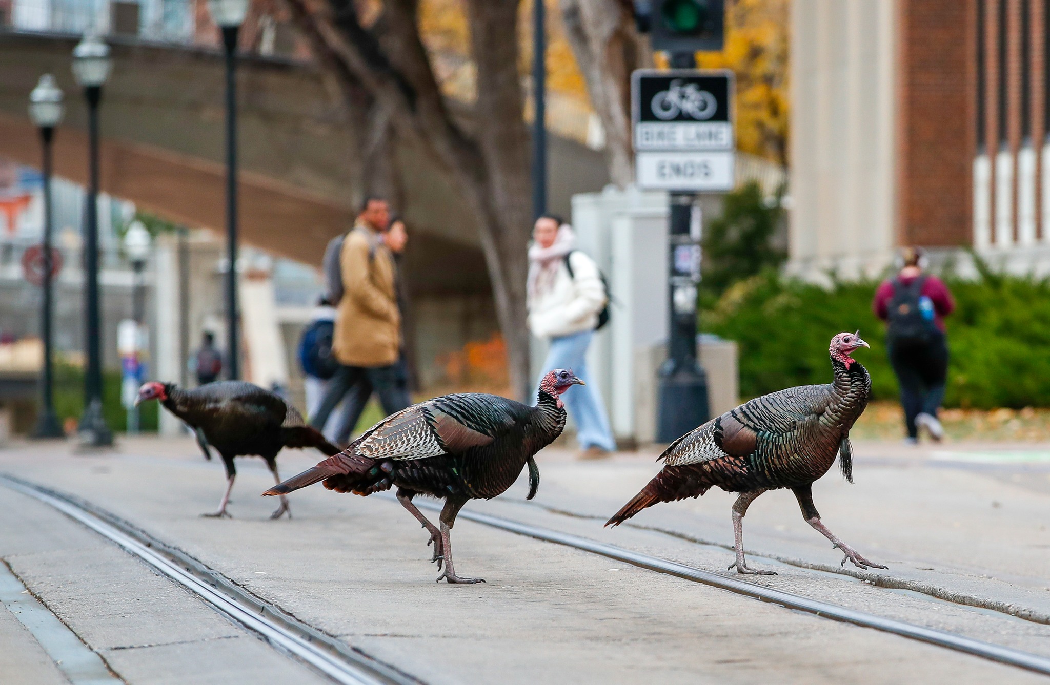
In the exponential population model, the growth rate depends only on the current population size . As a result, solutions with the same population value have the same slope, regardless of time. (See visiual aid in the Turkey Model below).
Today we will study autonomous differential equations more generally, using equilibrium solutions to understand long-term behavior. Later in the lecture, we will build on the exponential model by introducing the logistic growth model, which incorporates limiting effects on population growth.
Autonomous DE
A DE of the form is called autonomous. That is, when the independent variable is missing from the right hand side.
Example 1: The Turkey Model
The equation is an autonomous differential equation.
A constant solution of an autonomous DE is called an equilibrium solution.
Exercise
Find the equilibrium solutionsAn equilibrium solution of an autonomous DE is a constant solution. That is, a solution where is a constant. of the DE.
Steps
- Explain why and are both constant functions which satisfy the differential equation.
- Explain why no other constant function satisfy the DE.
If you’ve ever been to downtown Minneapolis, you may have seen turkeys roaming around. The DE above may be used to model the population of turkeys living in downtown Minneapolis, with representing thousands of turkeys and measured in years.
Pictorial Evidence
Logistic Growth Model
This turkey population equation is an example of a well-studied model, the logistic growth model:
Exercise
Rewrite the turkey equation to fit the standard form of the logistic growth model.
In this model, the population starts by increasing (or decrasing) at an exponential rate, but levels off when it reaches carrying capacity .
Visual Aid of Particular Solutions
Reflections
- Why do we generally ignore solutions below the horizontal axis for this model?
- Use common sense reasoning about the world to explain why the differential equation yields a reasonable model for the turkey population.
- Explain specifically why the equilibrium solutions make sense and how to interpret them in a real-world context.
- Compare your reasoning to the solutions in the visual aid. Does your reasoning appear to be reflected in the solutions shown?
Answer
Discussed in class. Mathematically, if and if
Exercise: Verify General Solution
Verify that is a general solution of the logistic growth model
Work in class
Students will begin with individual or collaborative work time, followed by a guided solution on the board developed through student input. Be prepared to explain your reasoning and contribute to each step of the process.
Final Exercise
In this section, we discussed general autonomous solutions, which arise in many applications. In particular, we spent a good bit of time analyzing the logistic growth model which exhibits exponential behavior unless it is near carrying capacity of the sytem, represented by , where it begins to level off.
- Modify the logistic growth model to describe a fish population being harvested at a constant rate. (Wildlife agencies and conservation scientists use models like this to help guide policies on stocking lakes, setting catch limits, and issuing fishing licenses.)
- Modify the logistic growth model to describe a panda population where is the smallest population size that can avoid extinction due to breeding difficulties and environmental pressures (). (Conservation biologists use models like this to study endangered species populations and determine when intervention is needed to prevent collapse.)
Solutions (Viewable in Posted Lectures)
- Fish Model: , where represents the number of fish being harvested for each unit of time.
- Panda Model: .
Some follow-up questions for the Panda Model.
- What is the sign of the derivative when ?
- What about when ?
- What do these derivatives represent for the Panda population in the model?
Exit Survey (time permitting)
On a blank sheet/slip of paper, complete the following sentences. Leave them on the front desk on your way out, and have a great weekend!
- Other students should ____________
- Other students should not ____________
- Dr.H should ____________
- Dr.H should not ____________
We’ll find some time next week to briefly go over the results! (beginning of Groupwork next Thursday?) If time did not permit, feel free to let me know your thoughts and suggestions either in support hours or anonymously in the folder on my office door.
Next Class
We’ll start solving differential equations analytically!